Why I Ditched malloc for AI Inference

In this post, I’ll show the impact poor memory management had on DSC, a tensor library I wrote from scratch in C++ and Python. I’ll then show how I fixed this by implementing a general purpose memory allocator from scratch. The goal here is not to implement something that is state-of-the-art or novel but rather to show what I went through when working on DSC and what I learned about memory management in the process.

Note: all the tests in this post were done on my workstation with a AMD Ryzen 9 3900X CPU, 64GB of RAM and an NVIDIA RTX 3060 TI GPU running Linux Mint 22.1 (Linux 6.8).

The Problem

During a single forward pass of Qwen2.5 0.5B, DSC is making over 2400 tensor allocations and deallocations. Below is a Perfetto trace obtained by running DSC with tracing enabled ¹ . Here, each pink spike shows either a tensor allocation or a deallocation ranging from a few microseconds to hundreds of microseconds and, in very few cases, even milliseconds.

This overhead compounds quickly but more importantly, this unpredictability can lead to random performance degradation. For example, consider a speed of roughly 100tok/s, this will give you around 10ms to generate a single token. In this case, a single 1ms spike in your memory allocator could lead to a 10% performance loss end-to-end.

Here’s how I eliminated all the malloc calls from the hot-path of DSC and how this led to better and more predictable performance.

The Naive Approach

When it comes to manually managing tensors, the most direct approach would be to naively call mallocand free whenever memory is required. If we want to deal with tensors on the GPU this involves also calls to cudaMalloc and cudaFree or equivalent. Also, we probably need a mechanism for sharing the underlying data buffer between tensors (see: Appendix A - Reference Counting), this could mean adding another object to the mix that wraps the raw data pointer and that is reference-counted.

One way of modelling our data is like this:

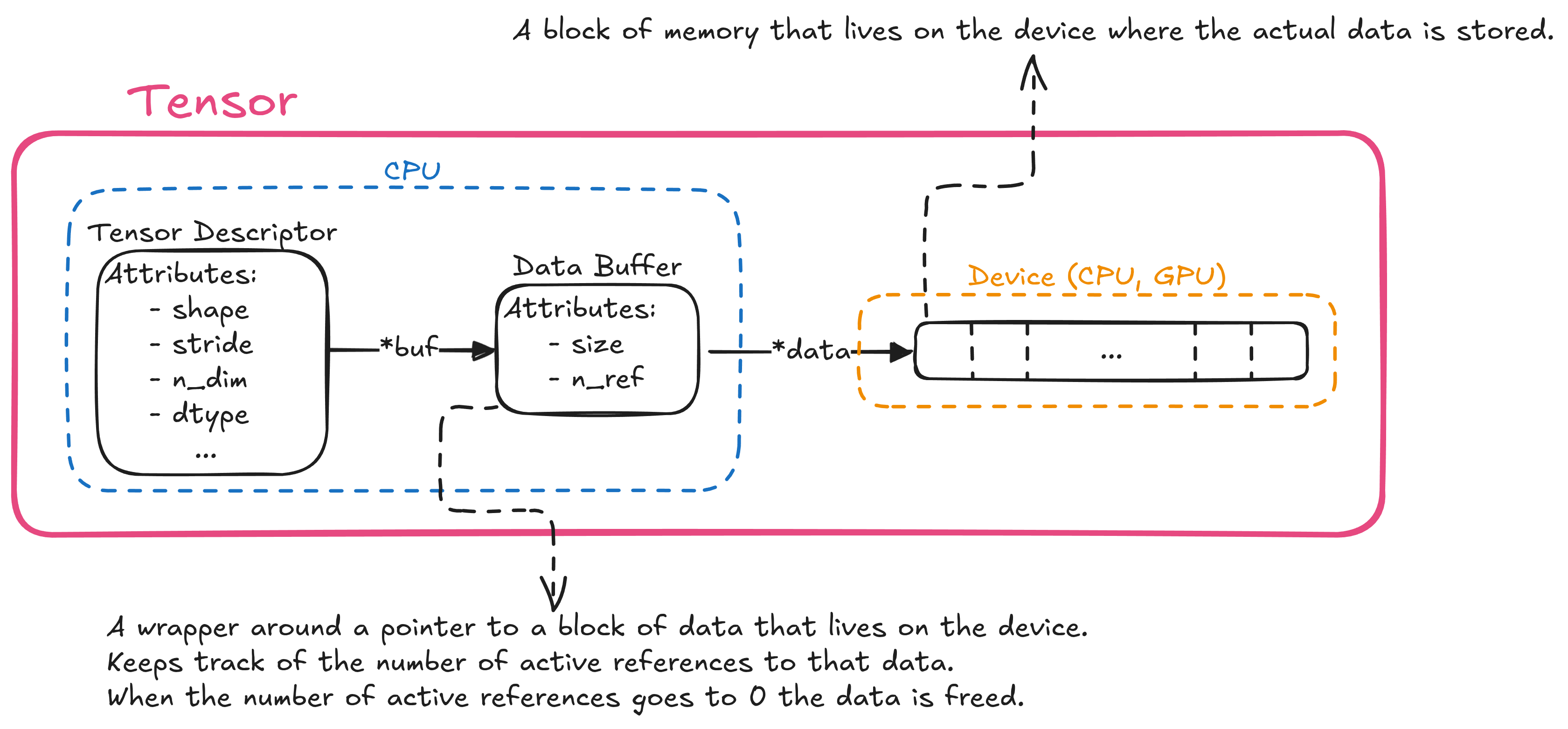
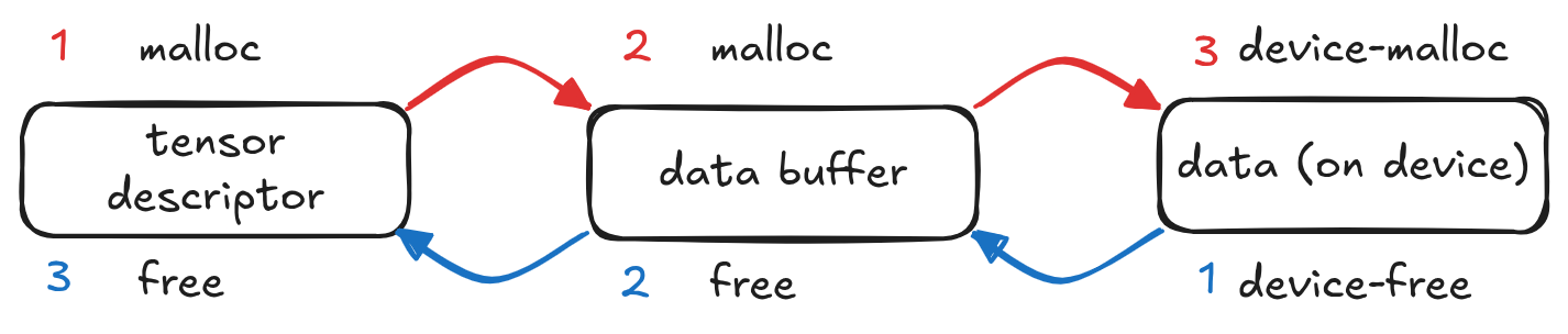
When it’s time to allocate a new tensor this is the workflow we expect:

1. malloc the tensor descriptor - the object that holds the tensor attributes like shape, stride and dtype
2. malloc the data buffer - the object that wraps the actual data pointer and is reference-counted
3. cudaMalloc the actual data block that lives on the device

Freeing is the same just in reverse order.

This pattern has to repeat twice for every intermediate tensor during inference. Matmuls need an output buffer, attention mechanisms spawn dozens of intermediate tensors for each layer and so on.

This could lead to a general performance degradation that is not easy to track ² and, most importantly, not easy to fix because this requires a complete redesign of how memory is managed in the entire application.

During my testing with DSC I found that memory allocations and deallocations account for 20-25% of inference time. This is pure overhead without any computational value. This number varies greatly depending on the size and complexity of the model (more layers = more allocations also, more complex operations = more intermediates = more allocations) but it also depends on how optimized everything is: if kernels get faster, allocations will account for even more of the inference time, becoming the real bottleneck.

Clearly, we can do better.

Step 1: Identifying Predictable Patterns

The key insight that made me change how I do memory allocation in DSC is that AI inference has very predictable memory patterns.

Unlike general-purpose applications that allocate wildly different object types and sizes, neural networks follow a simple template:

• Fixed model parameters: a few hundred to a few thousand tensors loaded once at startup and never freed
• Predictable intermediates: roughly the same temporary tensors created and destroyed in the same order every forward pass
• Large allocations: the unit of allocation is the tensor and that’s it. This means memory gets allocated in large chunks, so fragmentation isn’t a major concern

So, instead of asking the operating system for memory during inference, which is my hot path, I decided to do things a bit differently: allocate everything I need upfront and manage memory myself.

Step 2: Leveraging Predictable Patterns

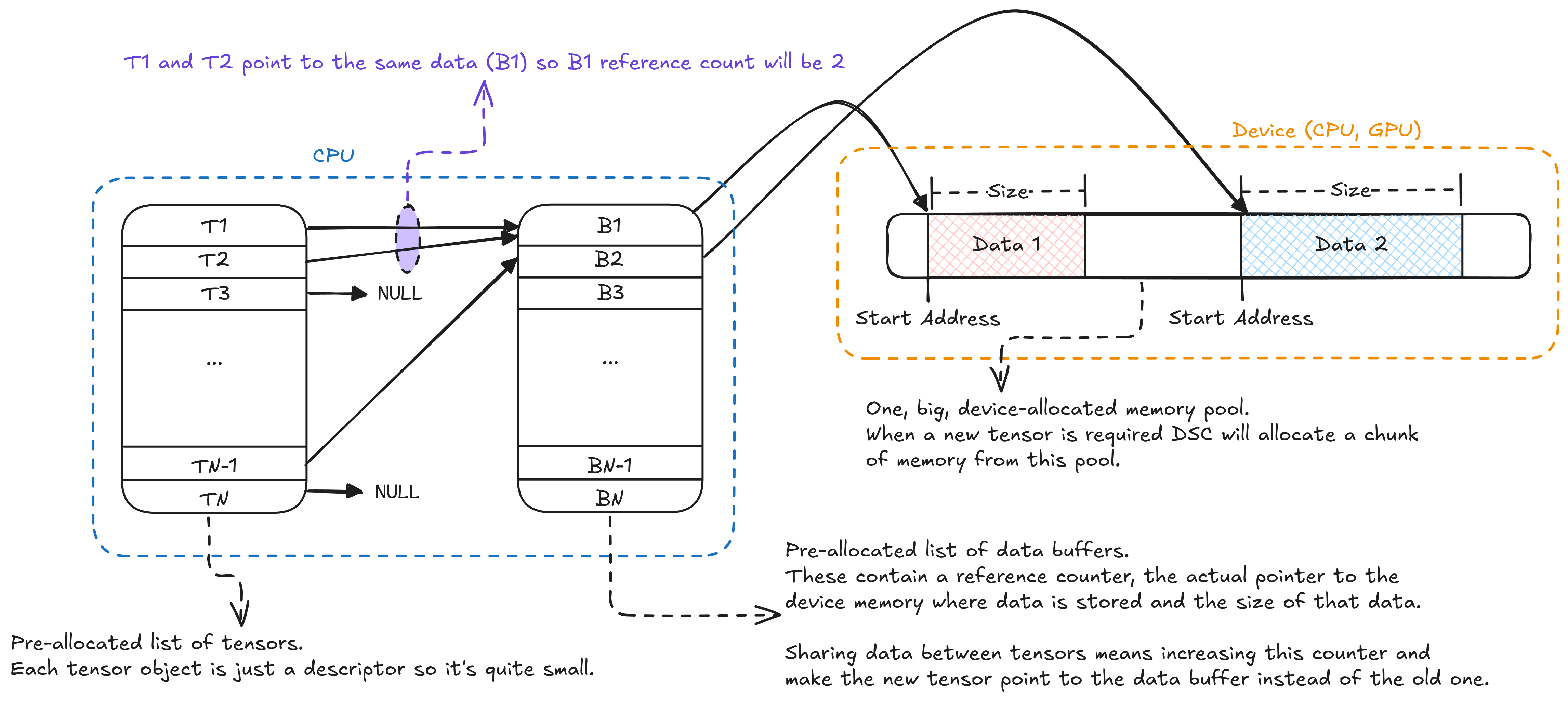
Instead of dynamic allocations everywhere, I switched to static allocations everywhere. At startup I allocate three things:

1. A static array of tensors descriptors - the objects that store the tensor attributes like shape, stride and dtype
2. A static array of data buffers - the objects that wrap the raw data pointer and have a reference counter
3. A large memory pool - one for each device (CPU, GPU) for the actual tensor data

This is what this looks like for the tensors descriptors:

struct dsc_ctx {
    dsc_device *devices[DSC_MAX_DEVICES];
    dsc_tensor *tensors[DSC_MAX_OBJS];
};

And this one is for the data buffers and memory pool:

struct dsc_device {
    dsc_data_buffer nodes[DSC_MAX_OBJS];
    // Actual pointer to device-allocated memory (ie. via cudaMalloc on NVIDIA GPUs)
    void *device_mem;
    // Alignment requirements
    usize alignment;
    // Extra device-specific information (ie. device name if GPU)
    void *extra_info;
    // How much memory this device has and how much of that is being used
    usize mem_size, used_mem;
};

Here’s the core insight: tensor descriptors are tiny objects that contain only a few attributes and there are only a few hundred to a couple of thousand of them active at any given time so I can just allocate all of them in a static array. Same goes for data buffers: they are even smaller (just one pointer and two integers for size and number of active references) so it makes even more sense to allocate them as an array ³ .

The actual data is managed through a simple memory pool per device. Instead of individual calls to cudaMalloc, I allocate one big chunk of GPU memory ⁴ at startup and manage it with a free-list allocator (see: #Appendix B - The Free-List Allocator).

This also has the added benefit of securing all the resources needed upfront: if there isn’t enough memory available the program won’t even start and will point this out clearly. This automatically gets rid of random out-of-memory errors during inference.

Allocation Becomes a Linear Scan

With this setup “creating” a tensor becomes trivial:

dsc_tensor *find_empty_tensor(dsc_ctx *ctx) {  
    for (int i = 0; i < DSC_MAX_OBJS; ++i) {
        if (dsc_tensor *x = &ctx->tensors[i]; dsc_tensor_is_free(x)) {
            return x;
        }	
    }
    return nullptr;
}

dsc_tensor *dsc_new_tensor(dsc_ctx *ctx,
                           const int n_dim,
                           const int *shape,
                           const dsc_dtype dtype) {
    int ne = 1;
    for (int i = 0; i < n_dim; ++i) ne *= shape[i];
	
    // Step 1: allocate the tensor descriptor 
    dsc_tensor *new_tensor = find_empty_tensor(ctx);
    DSC_ASSERT(new_tensor != nullptr);
	
    // Step 2 & 3: allocate the data buffer and the actual data
    new_tensor->buf = dsc_data_alloc(dsc_get_device(device),
                                     ne * DSC_DTYPE_SIZE[dtype]);
	
    // Fill tensor descriptor with shape, stride, dtype, ecc...

    return new_tensor;
}

That is: iterate through a (small) linear array and return the first tensor descriptor that is not currently in use, grab a chunk from the memory pool and return. Freeing a tensor is even simpler: notify that you no longer need memory for this tensor and mark your descriptor as available.

void dsc_tensor_free(dsc_ctx *ctx, dsc_tensor *x) {
    if (x == nullptr) return;
    if (x->buf != nullptr) {
        dsc_data_free(dsc_get_device(x->device), x->buf);
    }
    dsc_tensor_set_free(x);
}

The memory pool itself uses reference counting, so the actual chunk of data is freed only when the counter goes to 0. When that happens the chunk is placed back into the list of free blocks by the allocator.

The Drawbacks

This approach is obviously not perfect, there are several important drawbacks to keep in mind:

1. Higher upfront cost - all the allocations and setup need to take place during initialization, this could lead to longer startup times
2. Higher memory usage - the total amount of memory required by the system is larger than the naive malloc approach and can potentially become a bottleneck in constrained systems
3. Overall increased complexity - we are trading simplicity and speed of development for more control and better performance
4. Specialization over generality - while this implementation works very well for this particular problem it will not adapt easily to a different one. In contrast, the general approach of just using malloc will always work ok

While (1) and (2) depend on the physical constraints of your system and so they need to be evaluated objectively, (3) and (4) are more subjective. For me, they are worthwhile because:

1. Implementing this kind of algorithms with this very specific set of constraints is not that much more work and the performance and control gains could be huge
2. We’re trying to solve one specific problem, not chasing a moving target. This means we can afford a specialized solution

Regardless of what you decide to do, if you’re going to implement something that requires manual memory management, I strongly suggest you wrap your malloc and free calls in a well-defined internal API. This way it will be easy for you to change the implementation details (ie. opt-in something more performant like jemalloc). But if you sprinkle your code with random calls to malloc and free you’ll never even consider refactoring it because it will be too complex.

The Results

The impact of this new implementation was immediate and measurable:

• Faster and more predictable allocations
• Simpler debugging - no memory leaks or double-free issues
• Overall increased reliability - each call to malloc or free can potentially fail. By limiting those to only the startup phase of our application we increase the overall reliability of our system

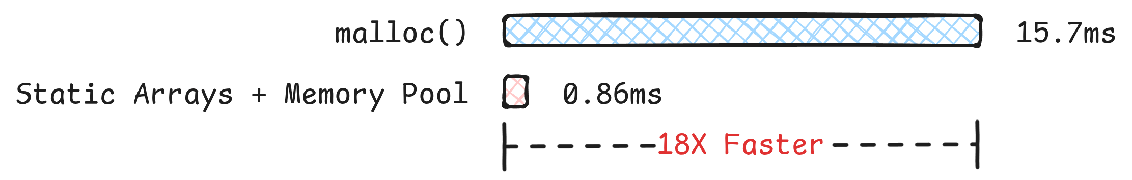
Here’s a side by side comparison of the naive malloc approach versus the new, static, approach:

	Naive malloc	Static Arrays + Memory Pool
Total inference time (1 token)	69ms	51ms
Total allocation overhead	15.7ms	862us
Allocation overhead	22.7%	<2%
Average latency (alloc)	2.4us	288ns
Average latency (free)	4us	66ns
Worst case latency (alloc)	184us	6us
Worst case latency (free)	1.276ms	1us

Conclusion

In this post I showed you how I removed all the malloc and free from DSC hot path by implementing a general purpose allocator from scratch that works surprisingly well.

The concepts we explored are not novel and are widely used: PyTorch for example uses mimalloc to handle CPU memory and a custom caching allocator for GPU. Regardless, it was fun for me “re-discovering” something on my own and finding that the same ideas (albeit with a lot more polish) are used in state-of-the-art systems like PyTorch.

Finally, I’d like to thank Jon and all the team over at HotAisle for giving me access to an 1x MI300X AMD VM to develop and test DSC. Your support has been invaluable. If you’re looking for some compute to run AI workloads or just try out AMD cards definitely check them out!

All the code discussed in this blog post and more is publicly available on GitHub.

---

Further Resources

There are a lot of good resources available online on the topic of memory management. The following is an incomplete list of resources I found useful when working on the allocator for DSC:

• I learned a lot about memory allocation in general from this series of posts by the gingerBill. The free-list allocator I implemented for this post is a modified version of what Bill presented in part 5.
• A very good article on the arena allocator in C by Ryan Fleury. Though DSC doesn’t use an actual arena the core lessons still apply.
• The original code of dlmalloc by Doug Lea in plain and readable C code. A modified version of this algorithm is used in glibc.
• Another very good article on the arena allocator by Chris Wellons.

---

Appendix A - Reference Counting

The term reference counting refers to a technique used to keep track of the number of active references to a resource such as a block of memory. It’s a very simple and commonly used technique for memory management. For example, it’s what C++ std::shared_ptr does to implement “automatic memory management”, it’s the main mechanism used in Python to implement garbage collection and is also used extensively to track objects in operating systems.

To understand how it works and why it’s useful when working with tensors consider this PyTorch-like snippet:

x = randn(4, 4)
y = x.view(16)

here we are creating a random tensor with some data associated to it. This is our “resource” and it has reference count = 1. Then, we want to create a new tensor that is just a flattened version of the first one without duplicating x. For this we create a new tensor y but, instead of copying the data from x, we just make y point to the same data as x. Now, our resource has a reference count of 2. The Python garbage collector will then keep track of x and y as if they are two separate entities the only difference is that when it’s time to free one of those instead of freeing the actual data buffer the reference counter is decreased. Only when the counter reaches 0 the data is actually freed.

Like all things, reference counting comes with some short-comings:

1. It requires every object to keep one extra field for the counter which causes overhead, especially if the size of the objects is very small.
2. The naive version I described above doesn’t work with reference cycles where an object refers directly or indirectly to itself. Such objects will always have a nonzero count and so will never be freed.
3. In a concurrent setting, all the updates to the counter must be atomic, which could introduce unwanted delays.

For our specific use-case (1) is not really an issue since we only need an integer (we could even use a uint8_t to save space) as counter for each data buffer that we have and since we only have a limited number of (usually very large) buffers the overhead is negligible ³ . (3) is not a problem either since we are not in a concurrent setting. We actually use multiple threads to speed-up CPU computations but this is just for computations, no allocation is made in the concurrent part of DSC.

The only real drawback is (2). But this is actually not a problem for our simple use case because we have the following constraints:

1. We have only 1 kind of object, the data buffer, that is reference counted
2. Data buffers can only reference data blocks, they can’t reference other data buffers. Also, each data block can have at most 1 data buffer pointing to it.

These mean that it’s not possible for us to have a circular dependency where two data buffers refer to each other.

In general, there are more advanced techniques that can be used to prevent this issue. For example, Python has a built-in cycle detector.

Appendix B - The Free-List Allocator

A free-list allocator is a general purpose allocator which doesn’t impose any restrictions. This means it allows allocations to be out of order and of any size. Due to its nature, the performance of this algorithm is generally worse than other, more specialized ones but this one is very simple and for our purposes is a good compromise for now.

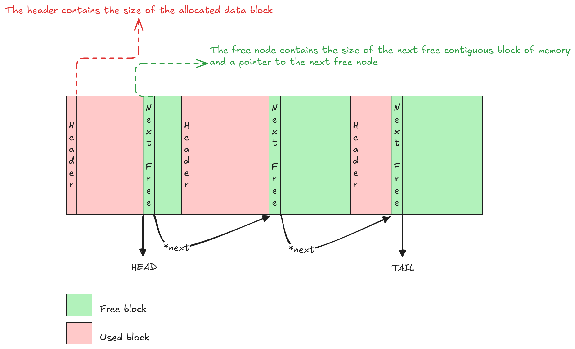
The idea is simple: keep a list of free contiguous blocks in memory along with their size. When memory is required, search through the list until you find a block where data can fit. If you find it, mark the data as used and remove the node from the free-list. To free data we must know the size of the data block to free and put that block of data back into the free-list. Finally, try to coalesce contiguous blocks of memory together to form larger free blocks.

We’ll see a free-list implementation that uses a linked-list to store the free data blocks. More efficient implementations are possible, for example using red-black trees, but those are more complex and generally not worth it for our simple use-case.

To allocate a new block of memory we have to go through the list of free nodes and find one that is large enough for our block of data. If multiple blocks satisfy this requirement we have to choose a policy: if we settle for the first block that works this is called first fit, if instead we decide to choose the block that works best (ie. the smallest available that fits) this is called best fit. The best fit approach can be a bit slower but it has the added benefit of reducing internal fragmentation.

Regardless, the time complexity for this operation is O(n), where n is the number of elements in the free-list.

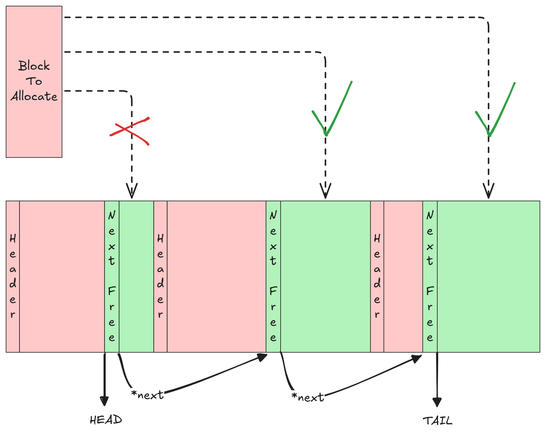
Once we allocate a free block, the free-list is updated and the now-used block is removed.

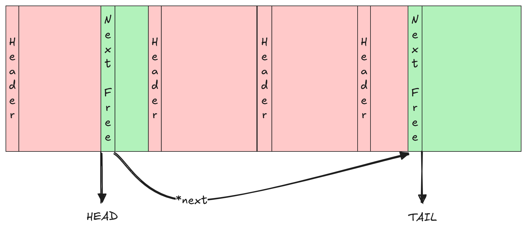
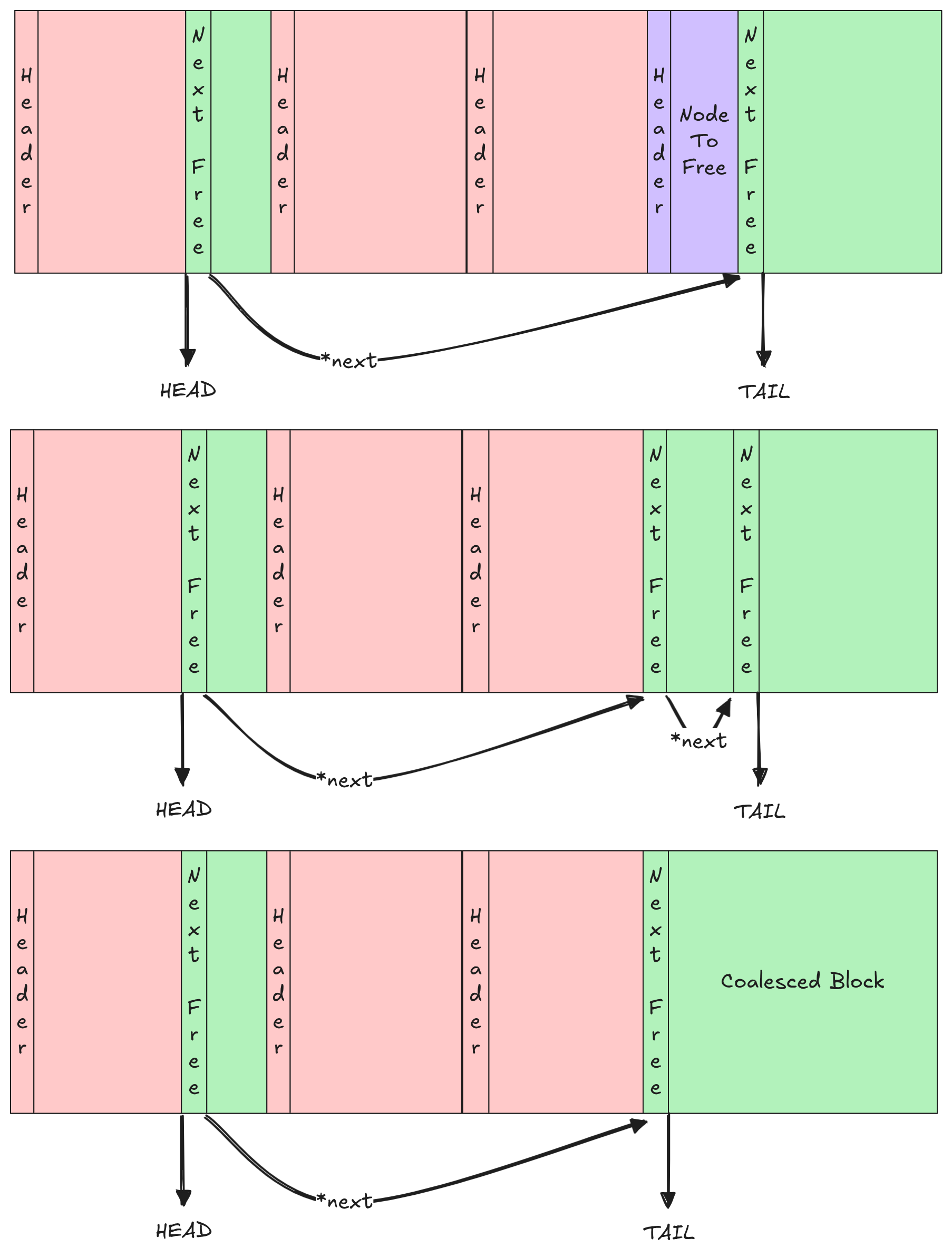
To free a previously allocated block of memory we just need to find its header. Then, iterate over the free-list until we get to the right position in memory order (this can be done by simply comparing the address of the block we are trying to free with those of the other blocks in the list) and insert the new node there.

When iterating, we have to store both the previous and next free nodes so that we are able to merge contiguous free blocks if possible.

As for the allocation process, the time complexity for freeing a block of memory is O(n), where n is the number of elements in the free-list, as we need to iterate over the list in order to insert the block in the right memory order.

The full source code of the actual implementation is available on GitHub.

---

_1. This trace has been obtained by compiling DSC in release mode with tracing enabled: make shared DSC_FAST=1 DSC_GPU=1 DSC_TRACING=1 and then running a single inference step of the Qwen2.5 0.5B model with this command:

TRACE=2 TRACE_ALLOC=1 python3 examples/models/qwen2_5.py \
"Can you write a quicksort in Python?" -n 1 --device=gpu --dtype=f32

Tracing in DSC works by capturing a CPU timestamp before and after a function exits, in this case the two functions we are looking at are: dsc_new_tensor and dsc_tensor_free.

_2. This is also referred to as “death by a thousand cuts”. One infamous example was in the Chrome browser where every keystroke triggered 250000 allocations due to an abuse of std::string (see: https://groups.google.com/a/chromium.org/g/chromium-dev/c/EUqoIz2iFU4/m/kPZ5ZK0K3gEJ).

_3. In practice, the value DSC_MAX_OBJS can be defined at compile-time with a default value of 1000. The actual dsc_tensor in DSC is exactly 56 bytes while dsc_data_buffer is 24 bytes. This means that we are “wasting” roughly 100KB of RAM (1 array of tensors, and 2 array of data buffers, one for CPU and one for the GPU) which is a very reasonable number, considering the kind of hardware required to run even the smallest models like Qwen2.5 0.5B.

_4. Currently, the size of the memory pool for each device can be configured at startup, when the dsc_ctx object is created. If a value is not specified DSC on GPU will take 90% of the total GPU memory.